Three Dimensional Iterative Scouring Methodology Using Commercial CFD Software
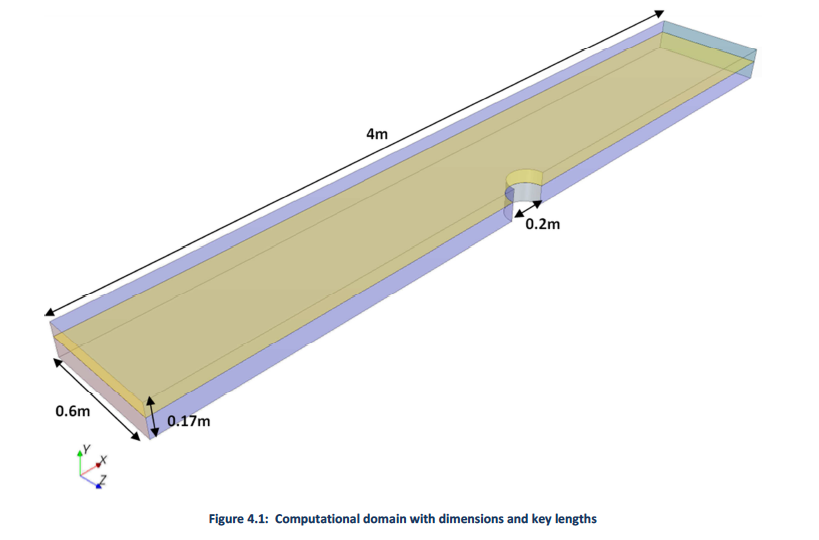
Offshore Center Denmark [1] conducted several experiments by varying the flow velocities and also provided a numerical model using FLUENT and compared the results. The results are limited to a very small (0.25mm) sediment size. The experimental setup consisted of a long rectangular flume with a cylinder in the center representing the wind turbine structure. The experiment was limited to cases where turbine supports were placed in ocean settings. Guo et. al [2] analytically determined the average bed and sidewall shear stresses for steady uniform flow in smooth rectangular channels. Their formulations show the importance of three main terms in the shear stress analysis: (1) a gravitational term; (2) a secondary flow term; and (3) a shear stress term at the interface. Van Rijn [3] experimentally determined sediment pick-up rate by using sediment lift installed in the center of the experimental flume. The sediment pick-up rate formula determined by him is used in the present study. In the previous phase of this project, Elapolu [4] developed a 3-D iterative methodology using existing commercial CFD software STAR-CCM+ to estimate a scour hole profile around bridge piers by moving the sediment boundary downward proportional to the supercritical shear stress. Results were compared to experiment data from Offshore Center Denmark. Simulations were limited to cases of a circular bridge pier and the critical shear stress at any point did not account for the slope of the bed. Guo [5] determined an approximate relation for the shear stress. His relation compares well with experimental results. His approximation is used in this study due to its simplicity
Mesh Morphing
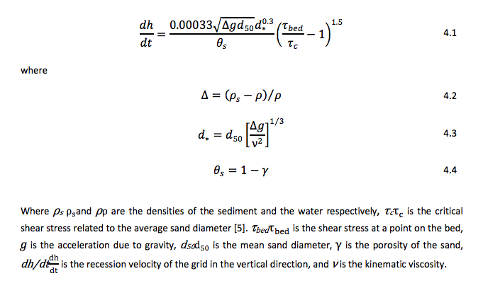

Where α is the angle between the sloped bed normal vector and the flat bed normal vector and ϕ is the angle of repose, taken as 33 degrees. The length of each time step is determined based on the maximum specified bed displacement and grid velocity, given by the following equation

where ∆ymax is the user specified maximum displacement for each time step and Δt is the length of each time step. In the following results a maximum displacement of 0.25mm is used. The maximum displacement per time step has been chosen such that it does not cause numerical instability. The scour bed displacement per time step is obtained by the following relation

is applied to displace each point on the bed where the shear stress exceeds critical at the conclusion of each time step. Mesh morphing after every time step propagates the bed displacements through the volume mesh. The mesh velocity that arises from the mesh morphing is included in the momentum and other transport equations, and therefore conservation law cell balances are maintained with the mesh morphing operation.
Simulation Results
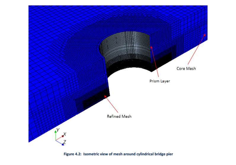
Found below are simulation results that use a mesh that does not fully capture the bed roughness height. Prism layers for the results below are 5mm, which would give an effective bed roughness height of 2.5 mm which is 1.125 times the average sand diameter. In practice, effective roughness heights would be 2 times the average sand diameter. Simulations with effective roughness heights are currently being run and those results will be presented at the next opportunity.
Figure 4.3 shows the scour hole formation using the variable critical shear stress (VCSS) and a constant critical shear stress (CCSS) approach, respectively. The scour hole is elongated in the wake region in Figure 4.3 (a), and has a more defined scour hole upstream of the cylinder. The scour hole is smoother and has steeper side walls in the VCSS approach than predicted by the CCSS approach. Steep side walls are not found in limited experimental results. Also, the maximum scour depth is larger and more area is scoured deeper using the VCSS approach. Red and blue areas represent no scour and deepest scour, respectively.
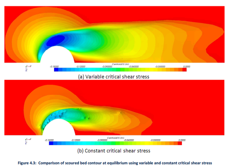
Figure 4.4 shows the evolution of the bed shear stress as it progresses from flat bed to equilibrium based on VCSS and CCSS approaches, respectively. Scouring begins after 10 seconds of simulation time; this allows a quasi-steady state condition to be established that is physically realistic before starting the transient computation. The VCSS case took approximately 50% longer in simulation time to reach equilibrium scour depth, but both cases ran in approximately the same clock time before equilibrium was achieved. The jaggedness in the curves are a consequence of remeshing, which does not preserve cell wall fluxes and property balances due to interpolation error in translating the solution to the new mesh. Use of the variable critical shear stress appears to yield a smoother evolution of the shear stress under the remeshing operation.
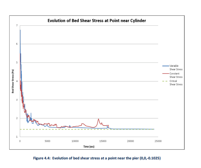
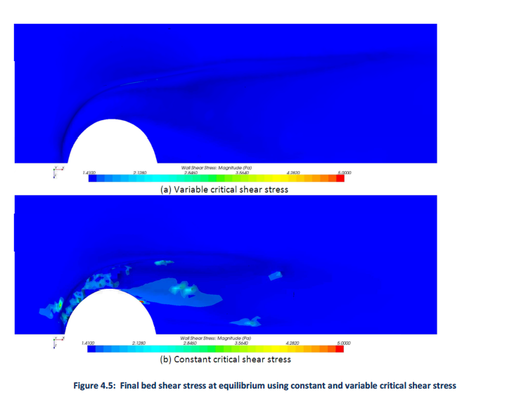
Figure 4.5 shows the bed shear stress at equilibrium using VCSS and CCSS approaches. The smallest shear stress value shown is 1.41 Pa, which corresponds to the pre-determined critical shear stress. There are still cells where shear stress is above the critical value, but the stopping criteria is taken at a point located at (0, 0,-0.1025) where the shear stress is below critical. There is still some very slow scouring occurring in the wake region of both cases, but nothing that would adjust the overall look of the scour hole or increase the maximum scour depth. Therefore, for all practical purposes, both cases have come to equilibrium.
References
1. Offshore Center Denmark. “Experimental Study of Scour around Offshore Wind Turbines in Areas with Strong Currents.” 2006.
2. Guo, Junke and Julien, Pierre Y. “Shear Stress in Smooth Rectangular Open-Channel Flows,” Journal of Hydraulic Engineering © ASCE / January 2005, 30-37.
3. Leo C. van Rijn, “Sediment Pick-Up Functions”, Journal of Hydraulic, Vol.110, No. 10, October 1984, pp.1494-1502.
4. Elapolu, Phani (2010). “Development of a Three-Dimensional Iterative Methodology using a Commercial CFD Code for Flow Scouring around Bridge Piers.” M.S. Thesis. Department of Mechanical Engineering, Northern Illinois University.
5. Guo, Junke (2002). Hunter Rouse and Shields Diagram. Advances in Hydraulic and Water Engineering, Vol. 2, pages 1096-1098.